Liberty File

The Liberty Timing file (Lib) contains detailed information on the timing and power consumption of the logic cells (std cells) of a cell library for a given technology node. In essence, Liberty is a timing model that includes data such as cell delay, transition time, setup and hold times, leakage power and more. This file, usually with the .lib extension, is a standard developed by Synopsys and distributed as open source. It is widely used in circuit design because it describes the characteristics of the cells, which are essential for timing analysis at several steps of the design flow.

Types of Liberty files

The timing and power parameters of a logic cell are obtained through electrical simulations run under different operating conditions — such as process, temperature and voltage variations. The results of these simulations are organized and stored in the so-called Liberty files (.lib), which EDA tools use for timing (STA) and power analysis. There are three main models used to characterize cells and generate these .lib files:

• NLDM (Non-Linear Delay Model)
• CCS (Composite Current Source)
• ECSM (Effective Current Source Model)

NLDM (Non-Linear Delay Model)

This is the most traditional and widely used model. In it, the cell is modeled with tables that relate the propagation delay and the output transition to two main parameters:

• Input transition (input net transition)
• Output load capacitance (Cload)

The simulations are run with voltage sources and the results are stored in 2D tables in the .lib file. The NLDM model is simpler and lighter, which means fast STA runs and smaller files. However, its accuracy is limited, especially in high-performance designs, where second-order effects have a bigger impact.

CCS (Composite Current Source)

A more advanced model, developed by Synopsys, in which the cell is characterized with a current source to model its electrical behavior more faithfully, including effects such as voltage drop (IR drop), coupling and waveform variations. The resulting file, called a CCS Lib, gives more accurate timing and signal integrity analysis and is ideal for more advanced technologies (for example, below 28 nm). On the other hand, CCS needs more input parameters, takes longer to simulate and produces larger .lib files.

ECSM (Effective Current Source Model)

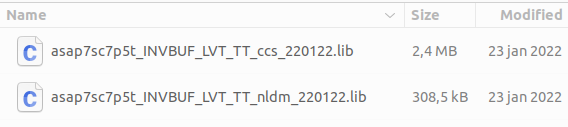
ECSM is an alternative to CCS, also based on a current source, but with a more compact and efficient model. It tries to balance accuracy and performance, giving results comparable to CCS with lower computational complexity and smaller files. ECSM is widely adopted by Cadence tools and stands out for accurately modeling the output waveform and internal transitions without hurting analysis performance as much. Each model has its pros and cons, and the choice between NLDM, CCS and ECSM depends on the accuracy, runtime and process technology requirements of the project. Figure 1 compares the size of a CCS file and an NLDM file.

Context in VLSI

In the integrated circuit design process, especially in logic synthesis and static timing analysis (STA), it is essential to have accurate information on the delays and power of the cells that make up the circuit, such as logic gates and flip-flops. Running SPICE simulations for the complete circuit would be far too complex and slow. That is why simplified timing models are used, which make it possible to estimate delays efficiently.

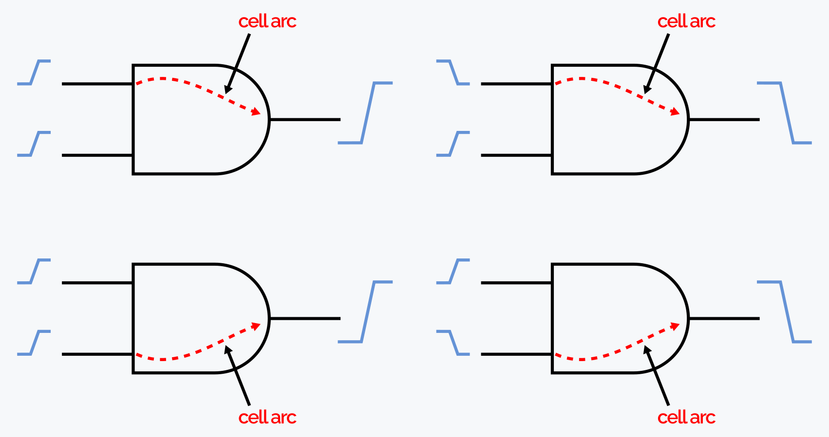
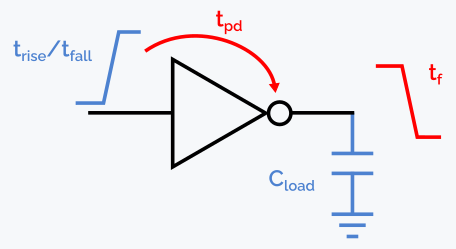
For each cell arc, that is, each specific path between an input and an output of a logic cell, as illustrated in Figure 2, two main parameters are determined: the propagation delay (tpd) and the output transition time (trise/tfall). The propagation delay is the time it takes for a change at the input to show up at the output. The output transition time indicates how long the output takes to settle after that change.

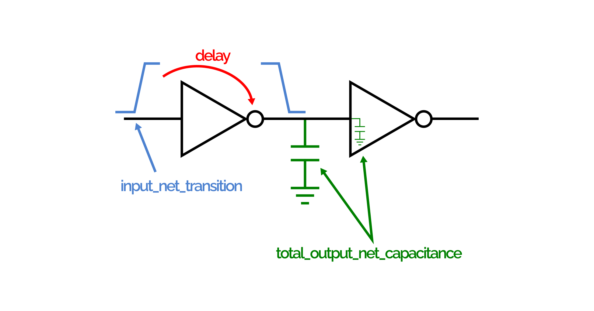
NLDM (Non-Linear Delay Models) are widely used for this purpose. They take two main factors as input: the input transition (input net transition, trise/tfall) and the output load capacitance (output load capacitance, cload). Based on these two parameters, which are tabulated in the .lib file, the EDA tools used for STA can compute both the propagation delay and the output transition, as illustrated in Figure 3 below.

The data in the Liberty file is provided by the foundry, which obtains it through detailed simulations during the electrical characterization of the standard cells. It is important to note that each Liberty file is generated for a specific set of operating conditions — process, temperature and voltage variations (called corners). So the propagation delay and output transition values depend directly on the corner used in the timing analysis.

Liberty is built from statements that may span several lines. All the information in a liberty file is described with three types of statements:

• Group Statements
• Attribute Statements
• Define Statements

Group Statements

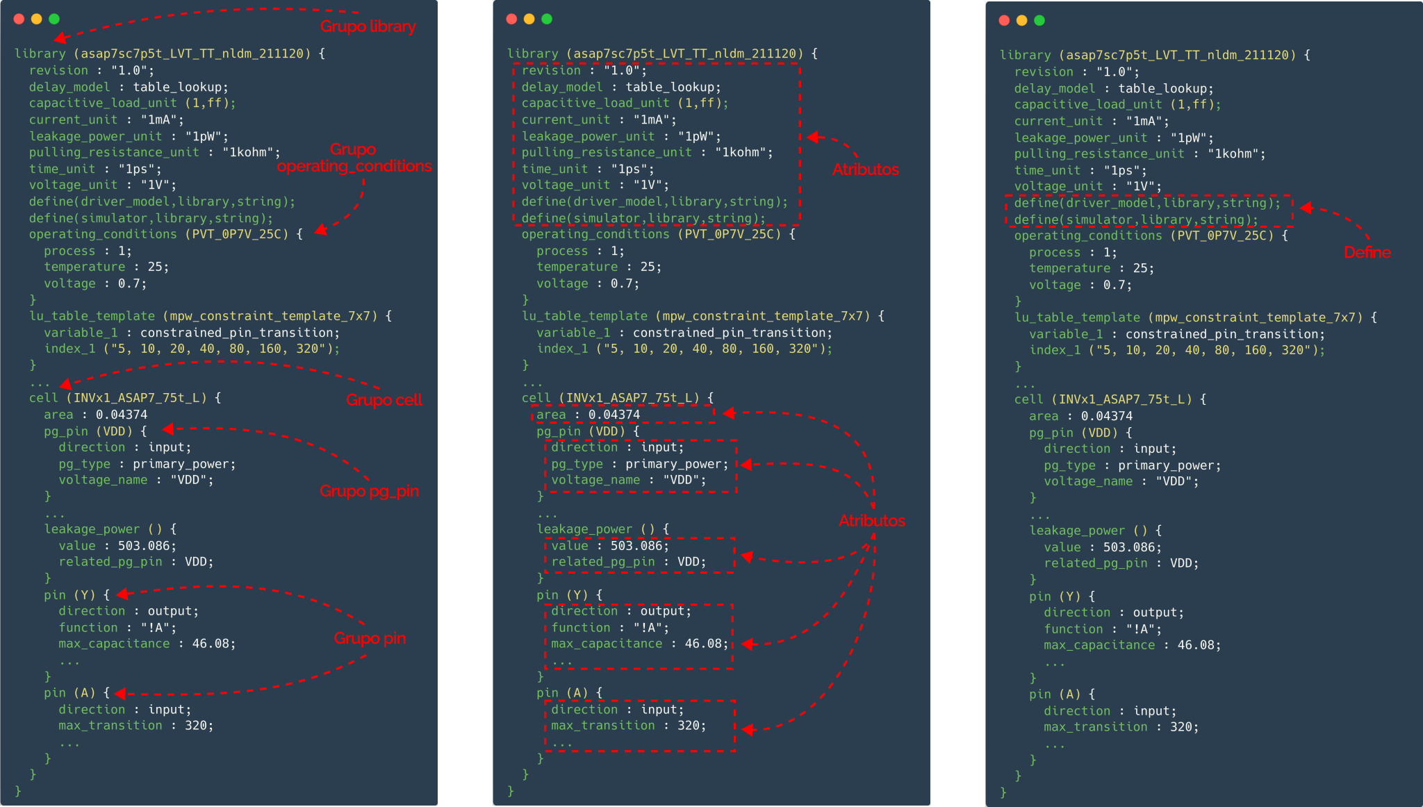
A group is a collection of statements that can describe a library, a cell, a pin, a timing arc and so on. Braces ({}) are used in pairs to enclose the contents of the group. A group can contain several attributes and even other groups as its elements.

    group_name (name) {
        … statements …
    }

Attribute Statements

An attribute statement sets a specific characteristic of a library object, such as a cell, a pin, etc. Attributes are always placed inside a group statement. Based on their syntax, attributes can be divided into two types: simple attributes and complex attributes.

• Simple Attributes

  Simple attributes have a basic syntax, regardless of the value. The attribute name must be separated from the attribute value by a space, followed by a colon and another space. Attribute statements must fit on a single line.

      attribute_name : attribute_value ;

• Complex Attributes

  A complex attribute includes one or more parameters in parentheses. The syntax of a complex attribute statement is:

      attribute_name (parameter1, [parameter2, parameter3 …] );

Define Statements

You can also create your own simple attributes with the define statement.

    define (attribute_name, group_name, attribute_type) ;

Large liberty files can strain disk capacity and memory. To reduce the size of the Lib file and make files easier to manage, the syntax lets you combine several source files. The references are made in the source file that contains the library group description. When the library is compiled, the referenced information is retrieved and included at the point of reference, and then compilation continues. The syntax of the include statement is:

    include_file (file_nameid) ;

Main Liberty fields

library group

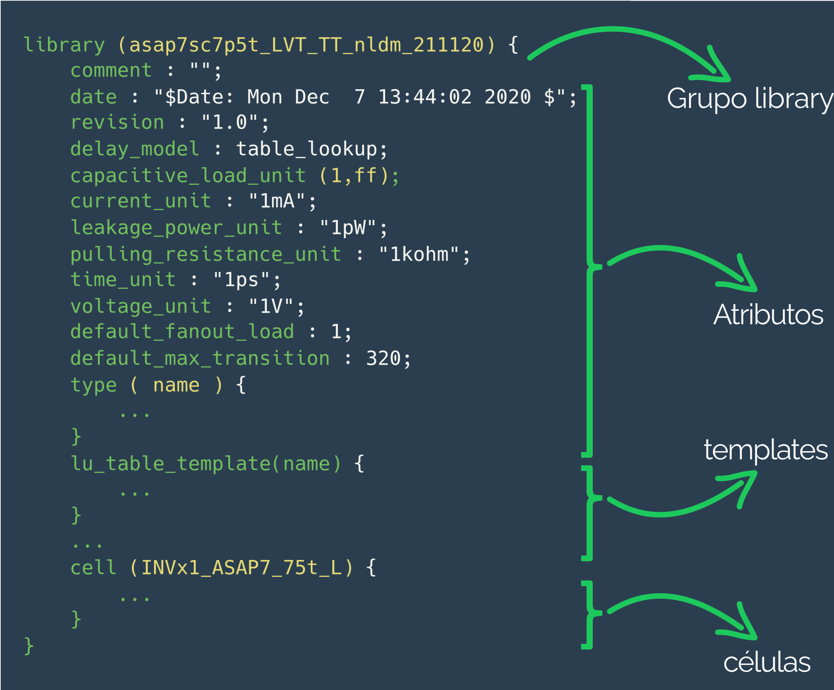
The library group defines the main structure of a Liberty file and covers the whole description of the cell library. All attributes and subgroups are organized inside this group. It is also at the library level that the global attributes that apply to every cell in the library are set. Each .lib file must contain a single library group, and its declaration must be the first executable line of the file. Figure 5 shows an example of how this group is declared in a Liberty file.

Templates

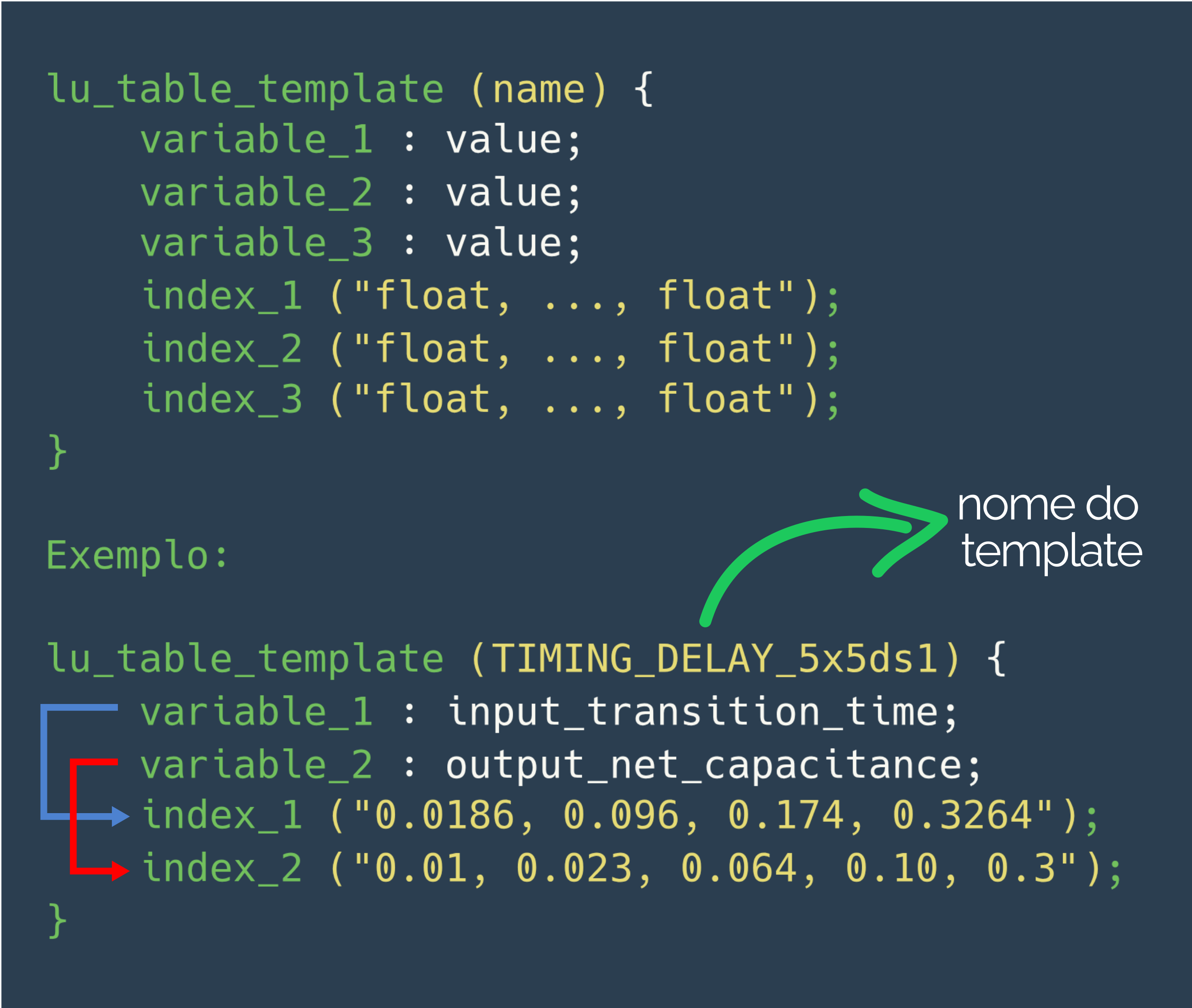
In a Liberty file, table templates are models that store common information reused by several lookup tables. Each template defines the lookup parameters and the breakpoints on each axis of the table. For a lookup table to use a template, the template must have a unique name. These table templates are especially useful to represent different kinds of timing delays and can have up to three variables: variable_1, variable_2 and variable_3. These variables indicate the parameters used to index the table data along its axes, such as the input transition time of a constrained pin, the output net length, or the output capacitance or load of a related pin. As shown in Figure 6, table templates help organize and reuse timing data efficiently.

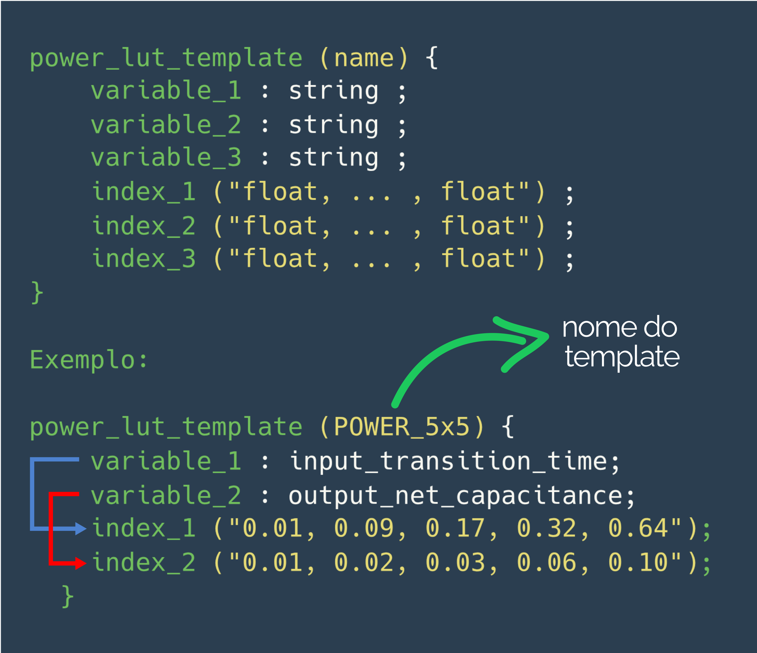
To represent the internal power of the cells in the Liberty file, you can also create reusable templates that store common information for several lookup tables. This is done with the power_lut_template group, defined at the library level (inside the library group). This kind of template specifies the table parameters and the breakpoints on each axis, as shown in Figure 7. As with table templates, each power_lut_template needs a unique name so it can be referenced by different power tables throughout the file.

cell group

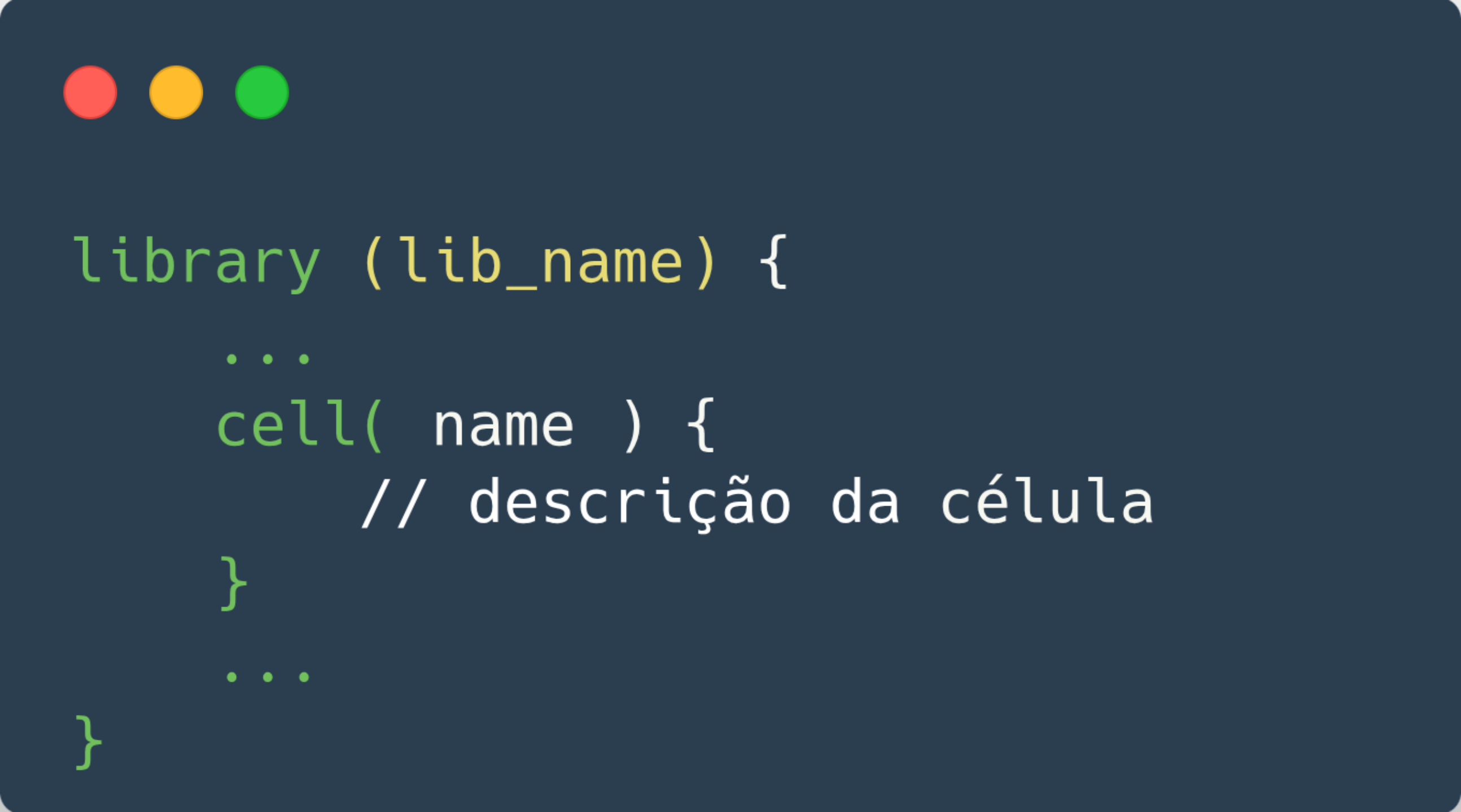
Cell descriptions are a fundamental part of a technology library. They provide information on the area, function and timing of each component in a given standard cell library. The cell group holds the attributes and groups that declare this information. Figure 8 shows an example of a cell group definition in a Liberty file.

pin group

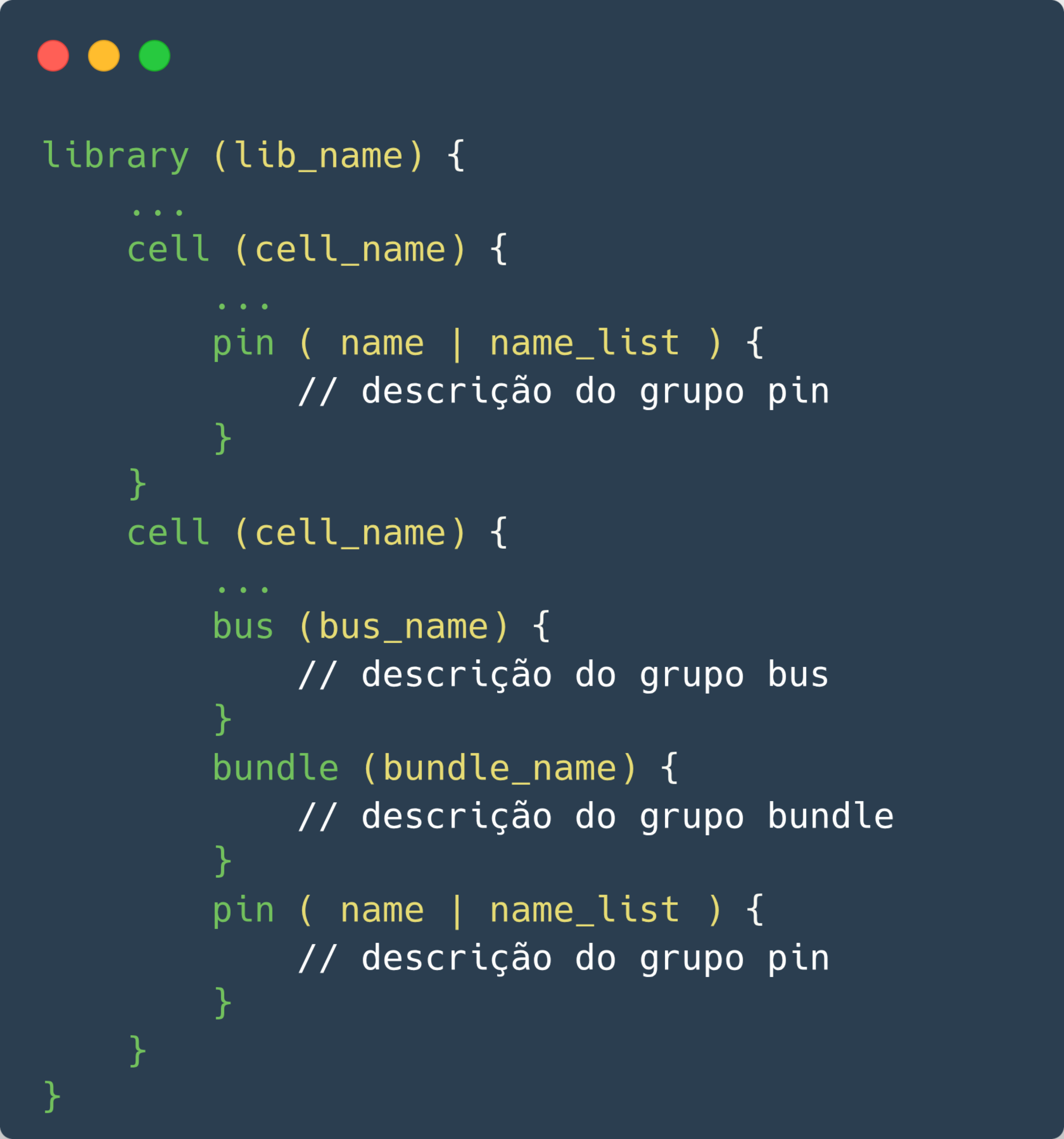
For each pin of a library cell, the cell group must contain a detailed description of that pin’s characteristics. These characteristics are defined in a pin group, which can be declared inside a cell, test_cell, model or bus group. Figure 9 shows an example of a pin group definition in a Liberty file, highlighting its main fields. The pin group usually includes important subgroups such as timing, which describes the delays and timing associated with the pin, and internal_power, which details the internal power consumption related to the pin.

Understanding Timing Arcs

Timing arcs, together with the interconnect information of the netlist, define the paths the timing analyzer follows while checking the critical paths of the circuit.

Each timing arc has a startpoint and an endpoint. The startpoint can be an input, output or input/output (I/O) pin. The endpoint is always an output or I/O pin, except for constraint timing arcs, such as setup or hold arcs, which can occur between two input pins.

All delay information in a Liberty file is associated with pairs of pins, such as input → output or output → output.

Combinational Timing Arcs

Combinational timing arcs describe the delay behavior of purely logic elements, such as AND and OR gates, inverters, etc.
This kind of arc is attached to an output pin, and the related pin can be either an input pin or another output pin. Depending on the transition type and behavior involved, the arc can be classified as: combinational, combinational_rise, combinational_fall, three_state_disable, three_state_disable_rise, among others.

These different types make it possible to model the circuit behavior in more detail, taking into account the specific rise and fall transitions as well as tri-state control.

Sequential Timing Arcs

Sequential arcs describe the timing behavior of elements with memory, such as flip-flops and latches. In these cases, when an arc describes the relation between a clock transition and the data output (input → output), it is treated as a delay arc. When it describes the relation between the clock and the data input (input → input), it is a constraint arc. The main types of sequential arcs are:

• Edge-sensitive (rising_edge or falling_edge)
• Asynchronous control (preset, clear)
• Setup and hold constraints (setup_rising, setup_falling, hold_rising, hold_falling)
• Non-sequential setup and hold (non_seq_setup_rising, etc.)
• Recovery and removal (recovery_rising, removal_falling, etc.)
• No expected value change (nochange_high_high, nochange_low_low, etc.)

These arcs are essential for analyzing timing constraints and data integrity in sequential cells.

Consider a simple combinational cell made of two inverters in series. This cell can be modeled in two different ways:

• Model A: defines two direct timing arcs, both starting at input pin A. One arc goes from A to Y and the other from A to Z. It is a simple, direct model.
• Model B: also defines two arcs, but more precisely. The first arc is the same as in Model A (from A to Y). The second, however, starts at output pin Y and ends at Z. This models more faithfully the impact of the load connected to Y on the delay seen at Z.

This kind of output-to-output arc can be used in both combinational and sequential cells, making timing analysis more accurate.

timing group

The timing group contains the information used to model timing arcs and trace paths during STA. It defines the timing arcs through a cell and the relations between the clock signals and the data inputs.

The timing group describes:

• Timing relations between an input pin and an output pin.
• Timing relations between two output pins.
• Timing arcs through a non-combinational element.
• Setup and hold times on flip-flop or latch inputs.
• Optionally, the names of the timing arcs.

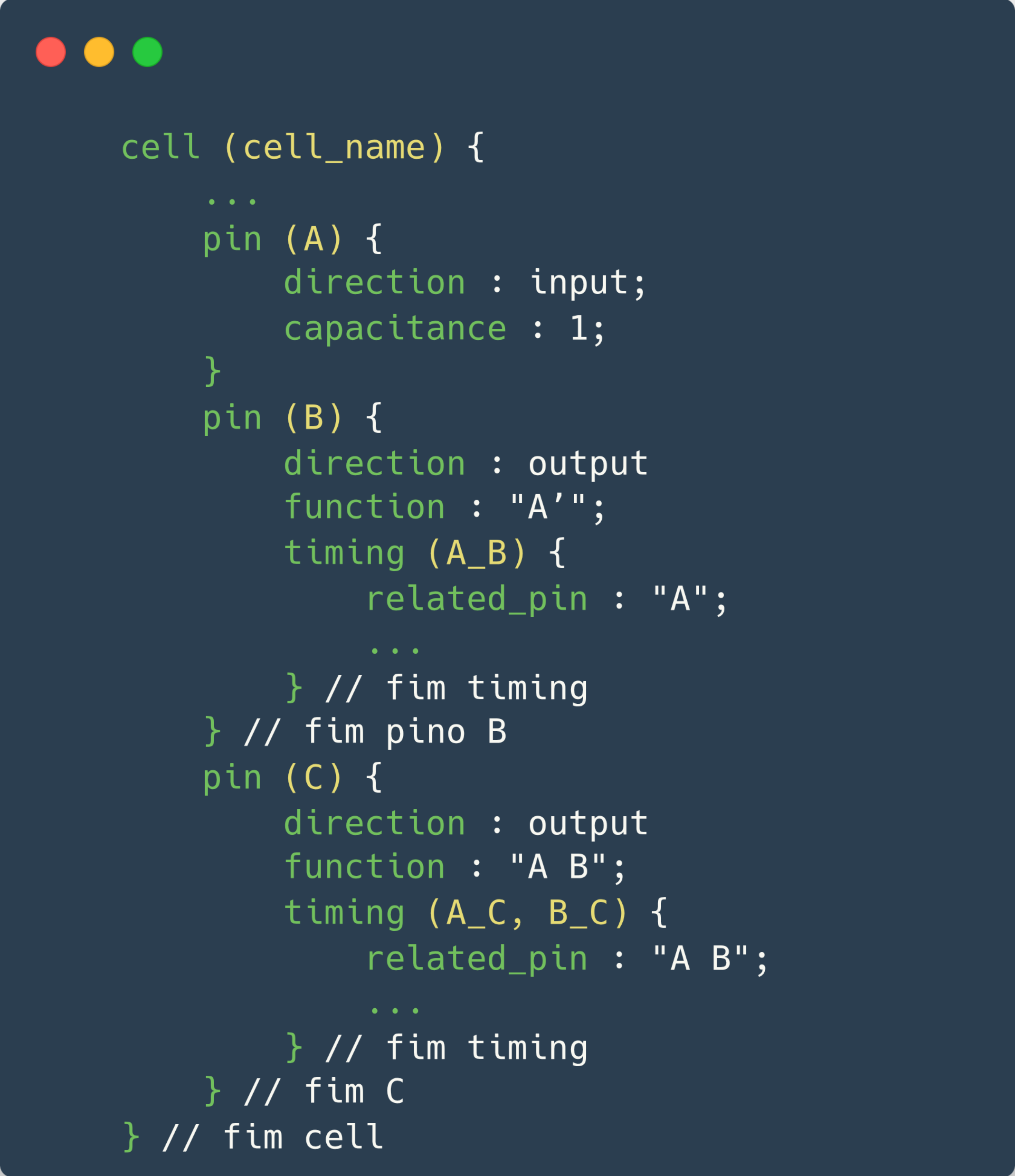
The timing group also describes setup and hold information when the constraint information refers to a pair of input pins. Figure 10 shows the structure of the timing group in a Liberty file, with its main fields and how they are organized inside the pin group.

Inside the timing group you can identify the name or names of different timing arcs. A single arc can occur between an identified pin and a single related pin, identified with the related_pin attribute. Multiple timing arcs can occur in several ways. The list below shows six possible configurations of multiple timing arcs:

• Between a single related pin and the multiple identified members of a bundle.
• Between multiple related pins and the multiple identified members of a bundle.
• Between a single related pin and the multiple identified bits of a bus.
• Between multiple related pins and the multiple identified bits of a bus.
• Between the multiple identified bits of a bus and the multiple pins of a related bus (with a given width).
• Between the internal pin and all the bits of the endpoint bus group.

Figure 11 illustrates these possible configurations of multiple timing arcs inside the timing group.

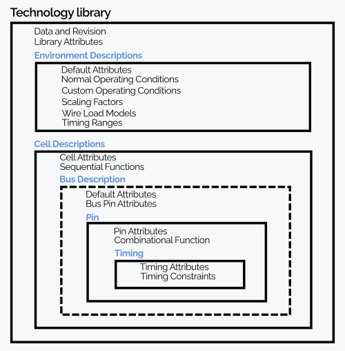
Now that we have explored the main elements of a Liberty file, we can represent its organization more clearly as a hierarchy, as shown in Figure 12. This visual representation helps you understand how the information is structured inside the .lib file, making it easier to read and navigate the different blocks of data, such as cells, pins, timing arcs and technology parameters.

Example of a delay calculation with the Non-Linear Delay Model (NLDM)

Suppose we want to compute the propagation delay (tpd) of an inverter (sg13g2_inv_1) in a library characterized with NLDM, shown in Figure 13. For that we need two input parameters:

• Input transition (input net transition): 0.174 ns
• Output load capacitance (Cload): 0.039 pF

These two values are used as indices to look up a delay table in the .lib file. The tables are usually 2D, with one dimension for the input transition and another for the output load.

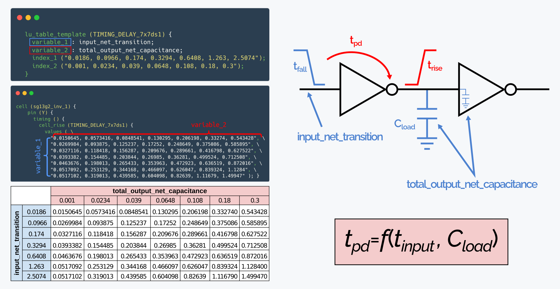
We find the indices in the table:

• Input net transition = 0.174 ns → middle row.
• Cload = 0.039 pF → middle column.

The corresponding value in the table is 0.0156287 ns, so the propagation delay (tpd) of the gate under this condition is 0.0156287 ns.

When the input values, such as the input net transition and Cload, do not match the points defined in the .lib tables exactly, EDA tools use interpolation. This makes it possible to estimate intermediate propagation delay values quite accurately from the closest tabulated data.

Design Liberty

Liberty files can also be generated for digital or analog blocks or IPs that have already been synthesized. This allows more accurate Static Timing Analysis (STA) at higher levels of the design, such as top-level integration. The information in these files depends on the timing constraints and specific requirements of the block, and it is essential to make sure the IP behavior is modeled correctly during timing analysis and the optimization steps of the final design.

Figure 14 shows an example of a Liberty file generated for a functional block (a counter), with its main information structured.

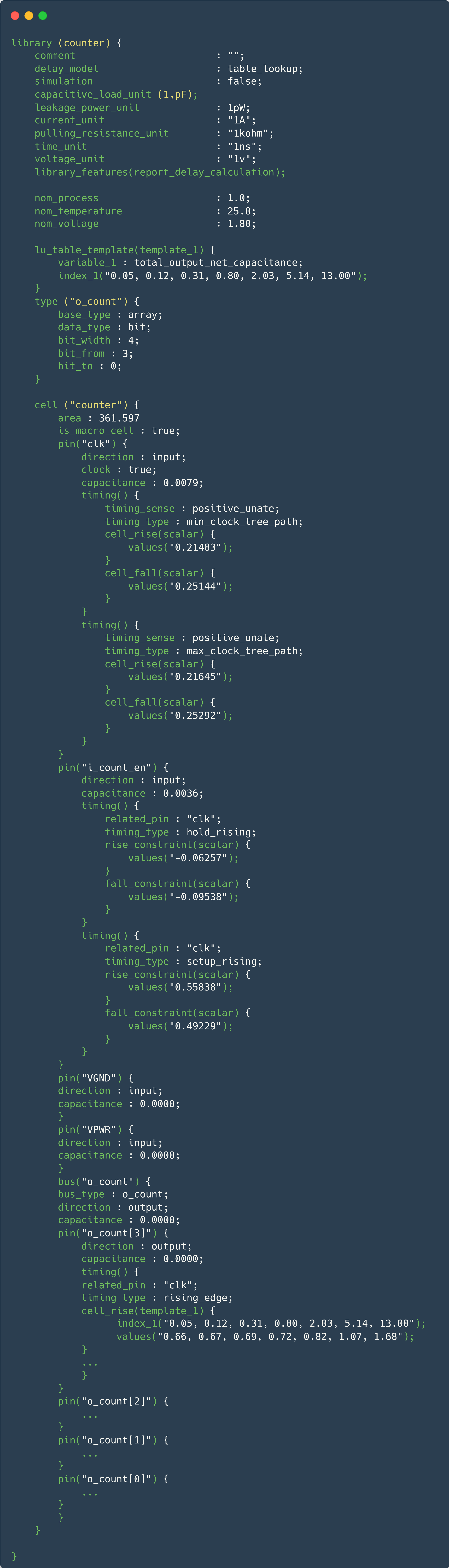
Usually, an IP that has timing constraints is characterized (memories, standard cells, custom digital blocks), and a .lib file is generated (with a Perl script or an EDA tool). If there are no timing constraints to meet, the minimum information in the .lib file is the pin section, without the timing/power sections.

An analog IP without constraints is usually delivered as LEF/Lib, and the .lib contains:

• Output pins (mandatory, consistent with the Verilog module)

• Maximum capacitance/transition/etc. values (design rules) (not mandatory, but they help placement/routing or synthesis fix and/or anticipate the capacitance value).

You can create a .lib by copying and pasting from an existing file and replacing the cell/pin sections, etc.

References

https://www.ispd.cc/contests/18/lefdefref.pdf. Accessed on 24-Jul-2023

http://coriolis.lip6.fr/doc/lefdef/lefdefref/LEFSyntax.html.. Accessed on 24-Jul-2023